A (very short) introduction to Python for Scientific Computations

This is a short introduction to the Python programming language, and the Jupyter format. This is a school on computational physiology and you will be using programming throughout to implement and solve various mathematical models, analyze the results and produce plots. Today we aim to give you a quick introduction and overview of Python and its syntax. If you are already familiar with Python, this can act as a quick refresher. As the school progresses you will have ample opportunity to use Python to solve various exercises, and get more experience and practice. If you are completely new to Python, don’t panic! We will have teaching assistants present to help you along.

The main topics covered in this session are:

• An introduction to Jupyter

• Variables and types

• Tests and conditionals

• Loops

• Plotting

• Defining functions

• Solving differential equations numerically

You can use this notebook to cover any of the topics more in detail than we get time for in the live session. Or you can use it as a reference later to refresh something.

If you want a more thorough introduction to scientific programming with Python, there are plenty of good books and courses out there, many of them open access. We can for example recommend the following open access book by Joakim Sundnes

• Introduction to Scientific Programming with Python

If there are any specific topics you want to learn more about, please do not hesitate to let us know, and we can try to cover these in more detail later in the course, or find you an appropriate source on the topic.

Parts of this material is based on an introduction to Python written Hans Petter Langtangen and Leif Rune Hellevik, which you can find on github.

Installing Python on your own Machine

For the lecture part of this school, you will mostly be coding and computing in the cloud through Jupyter. This means that you won’t have to install anything locally on your machine. If you want to also be able to run Python locally, for example for the project work in the course, you will need a Python installation. Let us therefore very briefly explain what you need.

Python is an open source project, and different implementations and versions exist. There’s also a many additional packages for scientific programmering we also want to install, such as FEniCS. Collectively, we refer to a given installation as a Python Environment.

Setting up and configuring a Python environment can be tricky for beginners, but there are good tools out there to help you. If this is all a bit new to you, we recommend you install a distribution specifically meant for scientific programming, so things are configured out of the box. We recommend using the Anaconda distribution. Downloading Anaconda will give you an up-to-date Python interpreter, many useful additional packages as well as a package manager you can use to download any additional packages you might need. You can download the Anaconda installer from

• https://www.anaconda.com/download/

Be sure to pick the version specific to your operating system (Linux/Windows/Mac OS), and select the newest version, i.e., Python 3.

If you are more experienced, feel free to manage your own Python environment whichever way you prefer, you could for example use pip or Docker.

Picking an Editor

In addition to a Python enviroment, you will need to install some sort of text editor to write your actual code in. Here plenty of options exist, some popular ones are

• Visual Studio Code

• Atom

• Sublime Text

• PyCharm

These are just some examples, and many, many more exist.

If you have installed Python 3 through Anaconda, you also get an editor called Spyder - as well as Jupyter (more on this shortly). And you can use this to write and execute Python code if you do not already have a preferred editor. Jupyter is mainly what you will use in this course, but again, you will use a cloud based version.

Spyder, and some of the other editors, are technically what we call an IDE (interactive developer environment), meaning it has a lot of added functionality in addition to being just a simple editor. Some people really enjoy these extra features, while others find them a bit distracting. You just have to follow your own preferences.

Figure: A Screengrab of the Spyder editor that comes with Anaconda. As Spyder is an IDE, it has quite a lot of extra features.

An alternative to using an IDE or a more minimialist editor, is to use Jupyter. Which is a tool that allows for combining your (executable) code with traditional text, images, mathematical equations and so on. It has become a very popular way to work with Python scripting, especially so for data science, where data can be explored and presented more interactively while working with the code itself. For your own project work, you can choose whether you want to use Jupyter, or more traditional scripts.

A Quick Introduction to Jupyter Notebooks

In Jupyter, files are known as notebooks, and are saved on your computer as .ipynb files. These are not traditional scripts or programs, but rather a combination of rich text, math, figures and code all contained in the same file. You interact with this file through your browser, which enables Jupyter to use HTML and other useful features. In this school you run on a cloud based Jupyter server, meaning the actual Python code isn’t run by your machine. If you install and run Jupyter locally on your machine, it will look exactly the same, and you still use your browser to interact with the notebook, but this time the Jupyter server is your own machine.

The Dashboard

When you start a new session, you will first enter the dashboard, where you can navigate to an existing notebook, or create a brand new one. Through the summer school, we have made one or more notebooks for each lecture session, which you can now access - or you can create a brand new one. We have tried to organize the lectures into a folder structure that is hopefully fairly selv-explanatory.

Note that when you access one of our notebooks, you get a local copy of this notebook. This means you can make whatever changes you want to the notebooks, and these will be saved for your user, but this won’t change the original, or anyone else’s notebook. Therefore, feel free to experiment and play around with code examples without fear of breaking anything. We will also give you exercises which you can solve directly in the notebooks.

Notebook Cells

The contents of a notebook are divided into a series of cells. A cell is a collection of content, and are split into two main types. Markdown cells contain content we associate with a typical text, such as written text, math, figures, tables and so on. Code cells contain code which can be executed, in which the output is written directly into the notebook, right below the code itself.

Example: Creating and running a code cell

Let us generate a code cell, write some code, and then run it. First we need to generate a new cell. Here you can either press the + button in the toolbar on the top, or simply use the keyboard shortcut b. This will generate a new cell. We see that the cell is a code cell, because it has the stylized In [] to its left.

You can now click the empty cell and start writing some Python code. Now, we haven’t started looking at Python code yet, so let us start with the simplest possible example, a print command:

print("Hello, World!")

Hello, World!

We have now entered some code into our cell. To run code inside the notebook, we must execute a given code cell. You can do this either by clicking the Run command in the toolbar at the top, or use the more efficient keyboard shortcuts Ctrl+Enter or Shift+Enter.

When you execute a cell like this, all the code inside the cell is executed and the output is printed immediately below the cell. In addition, the In []: will update to note which execution this was in the notebook, as this is the first cell we execute, it will become In [1]:.

print("Hello, World!")

Hello, World!

Execution order of cells

One element of notebooks that can be a bit confusing, to beginners and experts alike, is that a notebook is one big interactive session. This means that variables and results are remembered after running a cell, and can be used further down in a notebook, in different code cells.

However, when shutting down the notebook altogether and reloading it, this interactive data is forgotten. When opening a notebook, one can often not run a single cell in the middle or towards the end of the notebook, rather, one should run all the cells in the notebook from the start. A helpful tool here is to use the Cell > Run all option from the toolbar, which will run all cells in order, and load everything into memory. Alternatively you can use the Kernel > Restart and Run All if you want to completely reset and then run all cells in order.

If you start a new sessions in an existing notebook and execute cells out of order, you might get bugs or weird results - the typical example is simply error messages saying variables don’t exist as they have not been defined or imported (because an earlier cell that does this has not been executed). In weird cases the code might run, but the variables might not be was was originally intented, and so the results are off. Therefore: Remember to execute existing cells in order.

A more thorough introduction to Jupyter Notebooks

That was a very, very brief introduction to how to create code cells, write code and execute it in Jupyter. That is all you need to know for now to use Jupyter to write and run Python code. We won’t take the time to show you how to write other types of content in Jupyter for now, but you can look at our lecture notes written in Jupyter, or simply ask us, if you have questions. If you want a more detailed introduction to Jupyter, you can take a look at this guide to Jupyter basics by the original creators.

We now turn to the main topic of this session: coding in Python.

A Scientific “Hello, World!” Program

Traditionally, the first program one creates when learning a new programming language, is the so-called “Hello, World!”-program, which should just write out a message to the consol. In Python, this task is very easy, we simply use the print-command as shown above:

print("Hello, World!")

Hello, World!

The command print() is a built-in function that writes the output to the screen or console, or in this case, directly below the code cell.

There are a few important things to note in the code already:

• Because print is a function, we need to use parentheses when we call it.

• We put the function argument inside the parentheses. Functions can take zero, one, or multiple arguments.

• In this case, the argument is a text string, which we have to put inside either single- or double-quotes (' or "). These are equivalent, but you need to use the same character on both ends.

The “Hello, World!” program isn’t terribly exciting, so let us instead do a more scientific varient, where we compute some simple expression and write out the results. As a recurring example, we will use the following mathematical formula $\(s(t) = v_0 t + \frac{1}{2}at^2,\)\( Where \)s\( is the distance traveled by an object after time \)t\( with a constant acceleration \)a\(, starting with an initial velocity \)v_0$.

As an example, let us compute the distance travelered for \(t = 0.5\), \(v_0=2\) and \(a=0.2\).

t = 0.5
v0 = 2
a = 0.2

s = v0*t + 0.5*a*t**2

Here we first assign the three variables t, v0 and a. Note in each case the following

• We use the = symbol to define a variable

• The left-hand side is the name of the variable, while the right-hand side is its value

• More technically speaking, what is happening is that the assignment operation creates an object in memory, and the left hand side becomes a name for that object.

For the last line we are also defining a variable, by writing s = .... But in this case we de not simply hard-code in the value of this variable, but instead define it as the result of a mathematical computation. How is this interpreted by Python?

• Any time a variable is assigned, the right-hand side is first evaluated, and the resulting object is what is stored as the new variable

So Python computes the right-hand side, and stores the result in our s variable. But how do we figure out what the result actually is? We print it

print(s)

1.025

In this case we are not printing a text string, but a variable. Python then prints the value of the variable, in this case 1.025.

Note that s only stores the result of the evaluation. It does not remember “where it came from”. What we mean by that is that the formula itself is in no way remembered by Python. If you reassign t for example, the value of s does not change. You will therefore need to recompute s if you want to update it.

Your Turn

Repeat this example, but with the values \(t = 1.2\), \(v_0 = 4\) and \(a = -0.1\).

# Write your code here...

Also verify that the result does not change if you change one of the arguments after performing the computation.

Python as a calculator

Our scientific “Hello, World!” example contained a simple computation, and there are a few things worth noting:

• Standard arithmetic is written using the symbols: +, -, / and *

• Python has no implicit multiplication, we also need to write *

• Exponents use a double asterisk: **

• Python performs mathematical operations in the correct order.

Especially the last point is really useful for us, as it means we can simply write out the formulas as we would write it by hand, and Python we make sure it is computed correctly. You can of course add parentheses to affect order, which you sometimes should do. Other built-in mathematical operators that are useful are // for integer division, % for modulo, and abs(x) for absolute value.

Please also note that adding whitespace around variables and operators when writing mathematical expression does not affect the evaluation whatsoever. Therefore, feel free to add spaces in your equations to give them some space to breathe, which will make your code a lot more readable. For instance, we recommend to consistently put a space before and after the assignment operator (=), as it makes it a lot easier to read variable assignments.

Note on integer division

Note that dividing integers in Python 3 gives us a decimal (or a float-object to be precise). This is different to programming languages like C/C++ and also to Python 2. If you specifically want integer division, you need to use //.

print(2/5)
print(12//5)

0.4
2

Importing additional mathematical functions

The built-in operations only cover the most fundamental arithmetic operations. If we want more complex operations, such as roots, exponentials or trigonometry, we need to import this functionality. The standard package math contains all common mathematical functions, and if we need something a bit more rare, other packages exist that probably contain them, more on this later.

To import a function from a given package, you can write it as follows:

from math import sqrt

sqrt(81)

9.0

Or you can instead import the whole package as follows:

import math

math.sqrt(81)

9.0

There is third option, which is to import everything from a given package. This can be done by writing

from math import *

This is known as a wildcard import, the * means we want to import everything contained in the math library.

In general, such wildcards imports, where we import everything at once, is discouraged. This is because it becomes unclear what functions come from which packages, which can be a big problem for larger codes and programs. However, it is not uncommon to see it done in tutorials and the like, so it is useful to know about the option to do this.

Some of the functions contained in the math-package are

Function	Mathematical notation	Python
Square root	\(\sqrt{x}\)	sqrt(x)
Exponential function	\(e^x\)	exp(x)
Natural logarithm	\(\ln x\)	log(x)
Base-10 logarithm	\(\log x\)	log10(x)
Base-2 logarithm	\(\log_2 x\)	log2(x)
General base logarithm	\(\log_b x\)	log(x, b)
Sine	\(\sin x\)	sin(x)
Inverse Sine	\(\arcsin x\)	asin(x)
Hyperbolic Sine	\(\sinh x\)	sinh(x)
Factorial	\(n!\)	factorial(n)

Table: Common mathematical functions that can be imported from the math package.

A few things to note:

• All functions in Python are always called with parenthesis on the argument, even if the mathematical notion doesn’t always use this

• The trigonometric functions are defined in radians

• This list is not comprehensive. For a full overview of the math package, look at the official reference.

In addition to these functions, math also contains common constants, such as \(\pi\) and \(e\)

from math import pi, e

print(pi)
print(e)

3.141592653589793
2.718281828459045

Your Turn

Using Python as a calculator, compute the following expressions:

1. \(\frac{4\pi}{3}\)

2. \(12!\)

3. \(e^4 \cos(\frac{3\pi}{2})\)

# Your code here...

Scientific Notation

One final note on using Python to perform computations is that Python supports scientific notation which can be helpful when defining very large or very small numbers. Python has a useful shorthand for scientific notation, for example:

print(2.4e3)

2400.0

print(3.3e-4)

0.00033

Where 2.4e3 means \(2.4\cdot 10^3\), and 3.3e-4 means \(3.3\cdot10^{-4}.\)

Note that the same notation is sometimes used in output by Python as well.

print(6.4e2 * 5.2e-9)

3.328e-06

When doing physiological modeling, it is important to keep track of and be consistent in the choice of units, and using compact scientific notation can often be helpful to keep your code neat and readable.

Variables and Data Types

Let us return to our recurring example. The computation $\(s(t) = v_0 t + \frac{1}{2}at^2.\)$ We performed a computation by defining four variables:

t = 0.5
v0 = 2
a = 0.2
s = v0*t + 0.5*a*t**2

Here, we are defining the variables t, v0, a and s. Note that we do not have to declare the type of the variables as we make them, Python does this for us. This is different from some other programming languages like Java and C, where you always need to declare the types.

Even though we do note declare the types, note that any variable has a given data type. You can check the type of a variable with the type()-function.

print(type(t))
print(type(v0))
print(type(a))
print(type(s))

<class 'float'>
<class 'int'>
<class 'float'>
<class 'float'>

We see that v0 has become an int, meaning an integer variable, while the other three variables have become floats. A float is a decimal number, but because computers cannot accuretly represent arbitrary decimal numbers, we call them floating-point numbers because they have small inaccuracies.

There are many other types of built-in data types in Python. Some common ones, that exist in almost any programming language are

Name	Python type	Example values
Boolean	bool	True/False
Integer	int	4
Floating-point	float	3.1415
Complex number	complex	2.5 + 4j
Text String	str	Hello, World!

These are the most basic data types in Python, they each consist of one specific value. In addition, there are many built-in datatypes for storing collections of values (more on this later). Some of these are

Name	Python Type	Example
Tuple	tuple	(0, 0, 1)
Lists	list	[2, -3, 5, 8]
Dictionary	dict	{a: -9.81, v0: 5.2}
Set	set	set([2, 3, 5, 8, 11])

These built-in containers are useful for storing larger sets of data. They behave differently, so knowing what the different ones do is useful, but more on this later.

These examples are all built-in data types in Python, meaning they are available for use at all times. When you are using additional libraries and packages for Python, these usually introduce new useful data types. The most important one, by far, to be aware for our course is the package numpy (Numerical Python) which introduces a datatype called array. These represent mathematical vectors, matrices and tensors, and are extremely useful for performing larger linear algebra operations fast. We will therefore use the numpy package and its array data type a lot in this course.

It is also possible to define your own data structures through the use of classes, which is referred to as object-oriented programming, but we won’t cover this in this course.

Print Formatting

So far, we have seen how we can define variables, perform simple computations, and to look at the results using print. However, sometimes we want more control over how the output from print is formatted, we accomplish this through the process of print-formatting.

We have already seen that we can simply print variables to see their value

print(t)
print(s)

0.5
1.025

While this is very straight-forward and works well, we often want to write out a more descriptive message. We can do this by writing a string where we insert the values of given variables. This can be done through formatted strings, also known as “f-strings”.

print(f"After {t} seconds, the object has traveled {s} meters")

After 0.5 seconds, the object has traveled 1.025 meters

Note that we write a f (or F) immediately before the opening quotes of the string. When this is done, we can insert variables directly into the string with curly braces. When using f-strings, you can control more details on the printing of each individual variable by throwing on a format specification after the variable:

print(f"After {t:.2f} seconds, the object has traveled {s:.1f} meters")

After 0.50 seconds, the object has traveled 1.0 meters

Where we specify that we want the time written out with two decimals by writing (t:.2f). Here the f means that we are printing a float variable, and the .2 means two decimals. Similarly, we print out s with a single decimal.

When printing with a given number of decimals, Python will round our number for us.

x = 2.1436
print(f"{x:.3f}")
print(f"{x:.2f}")

2.144
2.14

Note that when rounding to three decimals, we round up, while for two decimals, we round down.

Python uses a convention known as bankers’ rounding, in which a .5 is rounded down if the preceding number is even, and up if it is odd. This is the standard way to round numbers for large data sets.

When using print-formatting, you can also write numbers out in different formats, such as scientific notation for example:

n = 41828
print(f"{n:.1e}")

4.2e+04

The format specificer .1e says that we want to write the number out in scientific notation with a single decimal.

Another specificer that is very convenient is g, as it will print the number out as a float for numbers close to \(1\), but for very small numbers, or very large numbers, it will instead use scientific notation. And another specificer to be aware of is the % specifier, which converts a decimal number into a percentage automatically. No need to manually multiply by a 100 anymore! Say we have performed 913 trials, with 642 succsessful trials, then we could for example write:

succsess = 642
total = 913
ratio = succsess/total
print(f"Succsess rate: {ratio:.1%}")

Succsess rate: 70.3%

More on Print Formatting

For more information on print formatting, you can take a look at this more comprehensive introduction.

Your turn

The volume of a sphere is given by $\(V = \frac{4\pi R^3}{3}.\)$ A normal football (regulation size 5 to be specific) has a radius of 11 cm.

Compute the volume of a football and print it out with a single decimal.

# Fill in your code here

If you did not convert units, your answer will be in cm\(^3\), but this is not a very intuitive quantity. Convert your answer so that it instead is printed out in number of liters, still with a single decimal. Recall that 1 dm\(^3\) is one liter.

# Fill in your code here

If-tests

An if-test allows us to endow our programs and code with logic, where it can check if some condition is met, and carry out special tasks only if something is a given.

The normal syntax of a simple if-test in Python is

if <condition>:
    <do something>

Here, <condition> is anything that can be evaluated to either True, or False. If the condition is true, then the code inside the test runs (typically called the if-block). If the conditional is false, the code is skipped and not executed. You can note which code belongs to a given conditional because it is given an indentation. The term indentation means the code lines are moved slightly in from the left hand side. This is acomplished by using the Tab key on the keyboard (or Shift+Tab to remove indentation). Most editors will however automatically add the indentation when you are defining a test.

The indented code block belongs to the condition, and will execute if and only if the condition is true. Any code lines further down without indentation will no longer belong to the test, and will execute no matter what.

Let us look at an example. Let us say we have a dataset of \(n\) samples, and we want to compute the median. If the number of samples is an odd number, then the median is simply the middle value, but if it is an even number of samples, we need to compute the average of the two middle values. To program an algorithm to find the mean, we must test if \(n\) is even or odd. We can do this with the following test:

n = 23

if n % 2 == 0:
    print(f"{n} is even")
else:
    print(f"{n} is odd")

23 is odd

In this example, we first define n = 23, this is just an arbitrary number, feel free to change it. Then we write a test to check if it is an even number. We do this by writing if n % 2 == 0. This might look like a very cryptic code at first, but let us break it down and understand it.

We write if <condition>: to make an if-test, so n % 2 == 0 is the condition we are actually testing. Here n % 2 means \(n\) modulo 2, which means the remainder we get if we divide \(n\) by 2. An even number is by definition any integer that evenly divides 2, meaning there will be no remainder. So only when n % 2 is equal to 0 will we have an even number. To check if two numbers are equal, we use double equality signs (==), this is common to nearly all programming languages and we do it because a single equality sign is used to assign variables.

When the if-test is encountered in the code, the condition is checked, but because n isn’t even, the condition is False, we can check this ourselves:

print(n % 2 == 0)

False

Because the condition is false, we do not execute the code that is indented under the if-test. However, we have also added an else-block, which will occur. Note that the else does not have its own condition, it simply happens if the condition is false. You do not always need to include an else, if there is no else and the given condition is false, then simply nothing happens, the code just skips the indented code altogether.

Other comparisons

In our example we checked if two numbers were equal with ==, but you can also check if two numbers are not equal with !=, or you could check whichever is larger or smaller than the other with < and >. For greater or equal you can do >=.

You can also combine several conditions with the and/or operators. The following test for example checks for a positive, even number:

n = 10

if n > 0 and n % 2 == 0:
    print(f"{n} is both positive and even")

10 is both positive and even

More than two outcomes

We have shown that you can use if-else to have two different outcomes for a given test. However, in some cases we might want to have more than two outcomes. In Python we can add more conditions to a given test by using the keyword elif. This somewhat cryptic keyword is short for “else if”. Say for instance we need to know if some number is positive, negative, or exactly zero, we could write it like this:

x = -2

if x > 0:
    print(f"{x} is greater than 0")
elif x == 0:
    print(f"{x} is exactly 0")
elif x < 0:
    print(f"{x} is smaller than zero")

-2 is smaller than zero

A given test can only have a single if and a single else, but as many elifs as you want. In either case, only a single block will ever be executed, if the first if-clause is true, then all the other elifs will be skipped.

If you want the different conditions to be checked seperately and independently. Then you simply use multiple if-tests in a row, but these will then be completely independent.

While Loops

We now turn to the topic of loops. Loops are one of the most fundamental concepts of programming, and are very useful tools to repeat an operation many times. In Python, we have two main kinds of loops, while-loops and for-loops. We start by looking at the while-loops.

A while-loop repeats itself as long as some condition is fulfilled. After each iteration of the loop, the condition is checked again. If the condition is still true, the loop is run again. If the condition is no longer true, the loop is finished.

The syntax of a while loop in Python is as follows:

while <condition>:
    <code block to be repeated>
    <code block to be repeated>
    <code block to be repeated>

There are a number of things to note with this syntax:

• We define the start of a loop with the keyword while

• We write in a given condition, and end the line with a colon (:)

• A set of indented statements follow the definition of the loop, these are the lines that repeat each time the loop is run again

The lines with indentation belong to the while-loop and we say ther are “inside” the loop. Any statements without indentation do not belong the loop, and will only be run after the loop is finished running.

Example: Computing \(s(t)\) over time

Let us look at an example. Returning to our recurring example: $\(s(t) = v_0 t + \frac{1}{2}at^2.\)\( So far, we have only computed specific values for a given \)t$. But say we instead want to print out a whole table of values, for different times. How can we do this?

Let us this time change the scenario so that we are looking at a ball thrown straight up, so \(a=-9.81\), and \(v_0=12\). We now want to compute \(s(t)\) over the first two seconds of the ball’s flight. We then need to decide on how many \(t\)-values we want to cover. Let us say we write out the net distance travelled each \(\Delta t =0.1\) s.

# Parameters
v0 = 12
a = -9.81

# Time
dt = 0.1 # Increment per time step
t = 0 # Starting time
T = 2 # Final time

# Loop
while t <= T:
    s = v0*t + 0.5*a*t**2
    print(f"{t:2.1f}  {s:4.2f}")
    t = t + dt

0.0  0.00
0.1  1.15
0.2  2.20
0.3  3.16
0.4  4.02
0.5  4.77
0.6  5.43
0.7  6.00
0.8  6.46
0.9  6.83
1.0  7.09
1.1  7.26
1.2  7.34
1.3  7.31
1.4  7.19
1.5  6.96
1.6  6.64
1.7  6.22
1.8  5.71
1.9  5.09

In this loop, the time variable t starts at 0, and the loop continues as long as teh condition t <= T evaluates to true. Each time the loop is repeated, we add increment t by dt. This means that every time the loop runs, t grows by 0.1, until it eventually reaches T and the loop ends.

In addition to incrementing t, the loop computes s(t) and prints both in a neatly formatted table. Note that we write the format specifies :2.1f and :4.2f. The number before the decimal point specifies the minimum width of characters to print. This is to keep the same column width.

Error in the code?

There is something a bit strange with our code. According to the definition of the while-loop, we should keep going while \(t \leq T\), and \(T=2\) s. This means the final pass of the loop should have t=2. However, in the last print, we see that we only get to \(t = 1.9\) s before the loop terminates. Why do we experience this behavior?

To understand this, we need to understand that computers cannot represent decimal numbers precisely, and so while what we want t to be 2.0, the increments of 0.1 have not been perfectly represented on the computer, and so t is ever so slightly larger than 2. We can see this by printing to machine precision by using 16 decimal places

print("{:.16f}".format(t))

2.0000000000000004

For this reason, we should be careful when we want to test or compare floats! Note that this is not a problem specific to Python, but rather a problem with limited precision of floating point arithmetic, and this is something we should keep in the back of our minds when working with numerical methods.

Example: Computing until the ball hits the ground

Here we used a while-loop to compute a table for the first two seconds, but we see that even at \(t=2\), the ball has yet to hit the ground again. Let us therefore change things around so we instead keep computing untill the ball hits the ground. This is as simple as changing the condition of the while-loop. We change this condition to while s >= 0. As soon as \(s\) becomes negative, we stop. However, now we also need to define some initial variable \(s\), so that the program can check the condition the first time the loop in encountered.

# Parameters
v0 = 12
a = -9.81

# Time
dt = 0.1 # Increment per time step
t = 0 # Starting time
T = 2 # Final time

# Loop
s = 0
while s >= 0:
    s = v0*t + 0.5*a*t**2
    print(f"{t:2.1f}  {s:4.2f}")
    t = t + dt

0.0  0.00
0.1  1.15
0.2  2.20
0.3  3.16
0.4  4.02
0.5  4.77
0.6  5.43
0.7  6.00
0.8  6.46
0.9  6.83
1.0  7.09
1.1  7.26
1.2  7.34
1.3  7.31
1.4  7.19
1.5  6.96
1.6  6.64
1.7  6.22
1.8  5.71
1.9  5.09
2.0  4.38
2.1  3.57
2.2  2.66
2.3  1.65
2.4  0.55
2.5  -0.66

We see that \(t=2.5\) is the first time step where the ball has gone below \(s=0\).

This second example illustrates one of the major uses for while-loops, as they can allow us to compute to some given condition, even if we do not know how many steps we need to get there.

Your turn: Using a while loop to calculate interest

Assume we have a savings account with an annual interest of 3.45%. If we deposit \(10,000\) to the account, how many years do we need to wait before the money in the account has doubled?

Fill in code below to answer this question. Hint: You will need a loop that looks something like this:

while <condtion>:
    money *= ...
    year += ...

The operators *= and += might be new to you. These are in-place operations that change an existing variable, so if you for instance write year += 1, the value of the year variable will be incremented by 1.

# Fill in code to answer the question

Lists and Sequences

Earlier, we mentioned that Python has built-in datatypes for collections of values. We will look at some of these now. Collections are useful for storing a set of data that naturally belongs together, for example a set of measurements. Different collections are useful for different things.

One of the more useful collections are sequences, often simply called lists. Lists are simply an ordered sequence of values. In Python, we can define such a sequence of values by writing them within square-brackets, and separating the different values by a comma

primes = [2, 3, 5, 8, 11, 13, 17]

Now, primes is a list variable. We say that it consists of 7 elements. We can find the length of a list with the function len(). We can also access individual elements as if they were individual variables through indexing by writing for example primes[2], the number in the brackets is the index. Note that Python starts counting at 0, so [2] would be the third element.

print(type(primes)) # Check the data type of the variable
print(len(primes)) # Print the number of elements
print(primes[2])  # Access an element by index. 

<class 'list'>
7
5

The use of len and indexing is not exclusive to Python lists, but can also be used on other sequence data types.

Appending elements

Python lists have a series of methods, special functions we can use to change the lists in certain ways. One example is the method .append, which we can use to add new elements to a list. We can for example start with an empty list, and build it up element by element.

Let us for example say we want a list of all powers of 2 less than 1000 $\(2^n < 1000.\)$ We could create these in a list by using a loop, and appending the elements one by one:

powers = [] # Empty list
n = 0

while 2**n < 1000:
    powers.append(2**n)
    n += 1

Here, the loop keeps incrementing \(n\) untill \(2^n\) grows beyond 1000. For each iteration of the loop, a new element is added to the list. To see the final list, we must print it:

print(powers)

[1, 2, 4, 8, 16, 32, 64, 128, 256, 512]

Other Useful List Methods

We see that we can use .append to add an element to the end of a given list. Such a function is called a method, because it acts on a specific object. All list-objects will have access to the .append() method. Lists also have a series of other useful methods we can use.

Method	Description
.append(value)	Add new element at end of list
.sort()	Sort the list in-place
.reverse()	Reverse the order of the list
.pop()	Removes the last element of the list, and return it
.pop(index)	Removes the element at a given index and return it
.remove(value)	Remove the first occurance of a given value in the list

Table:Useful methods for list-objects.

For a more thorough description of Python lists, and the methods, see the Python Tutorial, or the full reference on Python data structures.

For loops

We have briefly covered while-loops, now we cover for-loops. Where the while-loop repeats until a condition is met, the for loop goes through a collection of objects such as a list. We say that we loop over a list, or iterate through a list.

The syntax for a for-loop in Python is as follows:

for <element> in <sequence>:
    <codeblock to be repeated>
    <codeblock to be repeated>
    <codeblock to be repeated>

Here <sequence> should be some object consisting of several elements, for example a list. The <element> is a name we choose, this variable will be set to each element in the list as we loop, so that the loop repeats, but changing the active element each time.

We can for example loop through and print through the elements of our primes list

for p in primes:
    print(p)

2
3
5
8
11
13
17

Note that primes was a list we defined earlier, consiting of prime numbers. The variable p did not exist before we created our list, it is made by the loop itself. This is a normal point for confusion for beginners. Think of p as a mathematical variable that is equal to the different element of the list. Reading out the code as an english command also makes sense “for p in primes” is perhaps better understood if you read it as “for each element, p, in the sequence primes, do something.

In our first example, we simply printed out each element, which isn’t terribly existing. But let us instead perform something a bit more fancy, a small computation. We could for example explore Mersenne primes, which are on the form \(2^p-1\) where \(p\) is a prime, we could then do:

for p in primes:
    print(2**p-1)

3
7
31
255
2047
8191
131071

Or if we want to get a nicer table:

print(" p      2^p-1")
print("-------------")
for p in primes:
    print(f"{p:2} {2**p-1:10}")

 p      2^p-1
-------------
 2          3
 3          7
 5         31
 8        255
11       2047
13       8191
17     131071

Looping over Number Ranges

We have now see how we can use a for-loop to iterate through the elements of a sequence. However, often we do not want to loop over a list of elements we have already defined, but over some range of numbers. Take for instance our example above where we computed \(s(t)\) for a lot of different time points. Here we want to loop over a given set of numbers.

Now, one way to acomplish this would of course be to simply write out all the numbers:

times = [0, 0.1, 0.2, 0.3, ...]

But this would be incredibly boring and inefficient. Say we want to loop over one million numbers, it would simply be impossible to write them out.

Luckily, Python supplies a useful range function that creates predefined number ranges for us. The syntax is not terribly challenging, but it might take some getting used to.

Say we want to loop over the numbers \(1, 2, 3, ..., 10\), then we would do:

for i in range(1, 11):
    print(i)

1
2
3
4
5
6
7
8
9
10

A few things to note here is that range(1, 11) creates the range of integers starting at 1, but ending at 10 (not 11). Meaning the two arguments is the start, inclusive, and the end, exclusive. So range(a, b) gives what we mathematically would write as \([a, b)\).

Note that we have called our number i. This is just a normal convention when having a number that is counting upwards in integer steps. The convention comes from math, where one typically writes sums like: $\(\sum_{i=0}^{N} 2i - 1.\)$

To compute this sum in Python, we would need to decide on a specific \(N\), but then we could simply use a for-loop over the range and add each term to some summation variable:

N = 100

total = 0
for i in range(0, N+1):
    total += 2*i - 1
    
print(total)

9999

Note that we here wrote range(0, N+1), because we wanted to start at 0, and go up to and including \(N\). However, whenever we want to start a range at 0, we can simply omit it, this is just a handy shorthand, because we often want to start a loop at 0. So

range(0, N+1)

and

range(N+1)

are exactly equivalent. We also defined a variable total, this is because we need some variable to compute our actual sum. Note that while you might be tempted to call this variable sum, there is actually a function in Python called sum, and so you should refrain from using that name.

We can also add a third argument, in which case the syntax is

range(start, stop, step)

So the third argument says how the integer should increment. If we for example only want even numbers, we could do:

for i in range(0, 10, 2):
    print(i)

0
2
4
6
8

Your Turn

Use a for-loop combined with the range function, to write out a table of \(n\), \(n^2\) and \(n^3\) for \(n=0, 1, \ldots, 10.\)

# Fill in your code

Your Turn: Computing a sum

Use a for-loop to compute the sum of all integers from 1 to 1000, i.e., the sum $\(s = \sum_{n=1}^{1000} n.\)$

# Fill in your code for

Using a for-loop to compute \(s(t)\)

Earlier, we used a while loop to compute \(s(t)\) for certain time points. Let us repeat this exercise using for-loops. The main challenge now is that range only takes integer values, while we want to let \(t\) increase in steps of 0.1.

To get around this, let us say that \(t_i = i\cdot \Delta t\), so we let \(i\) count in integer steps from 0, and then we compute \(t_i\) and \(s(t_i)\) for each step. Earlier we printed out each value, but this time, let us append them to lists instead.

# Parameters
v0 = 12
a = -9.81

dt = 0.1
N = 21

t_list = []
s_list = []

for i in range(N):
    t = i*dt
    s = v0*t + 0.5*a*t**2
    
    t_list.append(t)
    s_list.append(s)

We have now stored the results in lists, we will use for plotting shortly. But for now, let us look at how we can use these lists to print out the nice table. Here we have two lists with the same number of elements, we can then loop over both at the same time by zipping them together with the function zip:

for t, s in zip(t_list, s_list):
    print(f"{t:3.1f}   {s:3.1f}")

0.0   0.0
0.1   1.2
0.2   2.2
0.3   3.2
0.4   4.0
0.5   4.8
0.6   5.4
0.7   6.0
0.8   6.5
0.9   6.8
1.0   7.1
1.1   7.3
1.2   7.3
1.3   7.3
1.4   7.2
1.5   7.0
1.6   6.6
1.7   6.2
1.8   5.7
1.9   5.1
2.0   4.4

Plotting

We now turn to a new topic: Plotting. Plotting is the process of producing graphics from numerical data. Plotting and producing graphics is a popular use-case for Python, and is especially relevant for scientific programming and data science.

Basic Python does not have access to plotting, and so we will need to import this functionality. Different packages for plotting exist, but we will use the most commonly used one: Matplotlib.

Matplotlib is a very popular, open source package for plotting. They have good introductions and examples on their website, and it is well worth a look. Matplotlib is very well developed and extensive for 2D plotting. If you want to make 3-dimensional plots however, some other packages are likely better.

To work with matplotlib, we first need to import it, here we start by importing the pyplot subpackage:

import matplotlib.pyplot as plt

We can now use plt. to access plotting functionality. The first thing we can do is plot our t_list and s_list against each other. The normal plt.plot command plots two sequences against each other, with the first along the x-axis, and the second along the y-axis. After calling plt.plot, we need to call plt.show to actually show the figure. Much like we often need to first compute a variable, and then print it.

plt.plot(t_list, s_list)
plt.show()

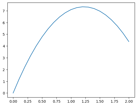
This curve is perhaps not all that exciting, but it shows our data in a intuitive way. However, the axis are not labeled, which we should fix! To do this, we use some additional commands between the plot and the show commands

plt.plot(t_list, s_list)
plt.xlabel('Time (s)')
plt.ylabel('Height (m)')
plt.title('Motion over time')
plt.show()

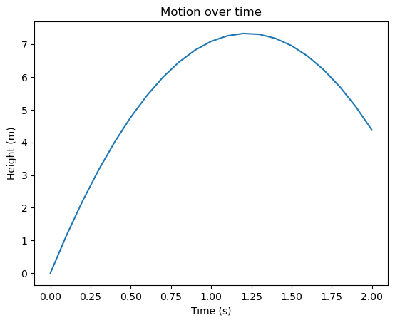
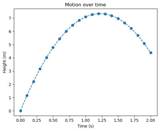
Even though are data set are explicit points in time, the curve is continious. This is because Matplotlib draws a straight line between each data point for us. We can plot this with a different line style to better show this if we want:

plt.plot(t_list, s_list, 'o--')
plt.xlabel('Time (s)')
plt.ylabel('Height (m)')
plt.title('Motion over time')
plt.show()

Using Numpy

The package NumPy (numerical Python) is very important if we want to do any kind of numerical computation in Python, and it can also be very helpful if we want to plot a mathematical function for example. In our \(s(t)\) example, we used a loop and lists to compute many points, but with NumPy, we can do this computation directly. First we import it

import numpy as np

Now we need to create a numpy array. These behave much like lists, but they are more mathematical in nature, and so we can do vector computations on them. This means we can simply write in the math, and the loops will happen behind the scenes, for us.

There are three main ways to define numpy arrays:

• np.zeros

• np.arange

• np.linspace

The first, zeros, creates an array full of 0’s, not very exicting. The arange works much like range, but it gives us a numpy array, unlike the normal range it can also take in decimals. The final one: linspace, stands for “linear spacing”, and it is used by writing np.linspace(a, b, n), and then it gives \(n\) linearily spaced points in the interval \([a, b]\).

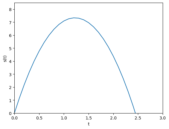
Using Numpy, we could compute \(s(t)\) as follows:

v0 = 12
a = -9.81

t = np.arange(0, 3.1, 0.1)
s = v0*t + 0.5*a*t**2

Now, t is not a number variable any more, but an array, or a mathematical vector if you will. Because of this, the resulting variable s is also such an array:

print(type(t))
print(type(s))

<class 'numpy.ndarray'>
<class 'numpy.ndarray'>

plt.plot(t, s)
plt.xlabel('t')
plt.ylabel('s(t)')
plt.show()

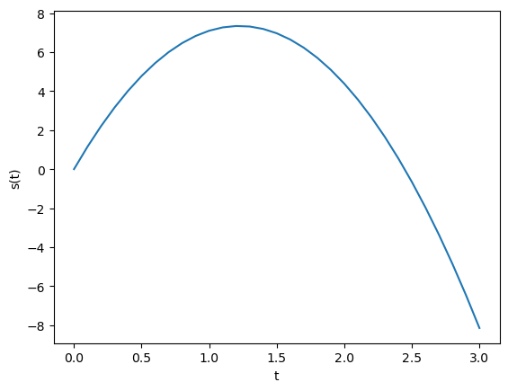
Here \(s=0\) represents the ground, so the automatic axis becomes a bit weird. We can control this using plt.axis([xmin, xmax, ymin, ymax]):

plt.plot(t, s)
plt.xlabel('t')
plt.ylabel('s(t)')
plt.axis([0, 3.0, 0, 8.5])
plt.show()

Numpy also provides all the normal mathematical functions that works with vectors. Say for instance we want to create a sine curve, we can do it as follows:

x = np.linspace(0, 4*np.pi, 50)
y = np.sin(x)

plt.plot(x, y)
plt.xlabel('x')
plt.ylabel('sin(x)')
plt.show()

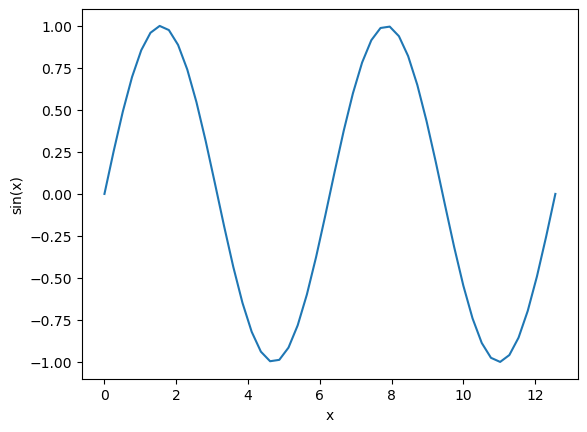
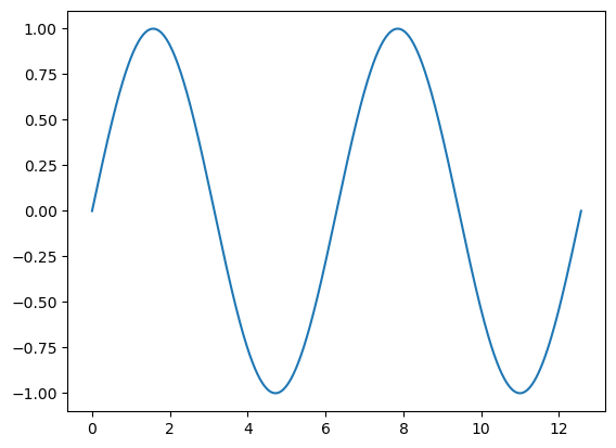
With only a few lines of code, we produce a nice sine curve. Note that we use linspace to plot two whole periods (from 0 to \(4\pi\)). The curve looks nice except that the tops look a bit jagged. This is because we compute too few points for it to look completely straight. Let us upp the number of points:

x = np.linspace(0, 4*np.pi, 1001)
y = np.sin(x)

plt.plot(x, y)
plt.show()

Numpy also has other common mathematical operations available in vectorized versions, including log(), exp() and sqrt(). Normal arithmetic operations also works well with arrays

Your turn: Plotting a damped sine wave

Make a program that plots the function \(g(y) = e^{-y}\sin(4y)\) for \(y\in[0, 4]\).

Your turn: Plotting a circle with parametric representation

Use np.linspace to define \(\theta \in [0, 2\pi]\), and then let \(x = \cos(\theta)\) and \(y = \sin(\theta)\). Plotting \((x, y)\) should now give a circle. Use plt.axis('equal') between your plot and show statements to make the dimensions of the \(x\) and \(y\) equal.

Other kinds of plots

We have only shown the command plt.plot so far to plot out curves. However, matplotlib supports more or less any kind of normal 2D plot. Some popular matplotlib plotting commands are

• plt.bar for barplots

• plt.scatter for scatterplots

• plt.hist for histograms

• plt.contour for contour plots

• and so on…

There are way to many possiblities to list here.

We recommend you look at the Matplotlib example gallery to look for inspiration. For any kind of plot you can click it to see example code used to generate it.

Defining Functions

So far, we have used a lot of functions, for example print, sin, np.linspace, plt.plot and so on. All of these are functions we can call on to perform specific tasks. Now we will look at how we can define our own functions.

The benefit of defining our own function is that we can avoiding the same code many times over. This is more efficient, and easier to fix if something is wrong. It also makes our code more structured and easy to understand, as a function is a form of abstraction. If we write a function that performs some given task, we can later on rely on that function while no longer having to think about exactly how that task is achived. This is a big benefit, because the human mind is not good at focusing on too many different things at once.

Let us show an example. What better example than our trusty function: $\(s(t) = v_0t + \frac{1}{2}at^2.\)$ To define this function, we write:

v0 = 12
a = -9.81

def s(t):
    return v0*t + 0.5*a*t**2

Here you can note especially that:

• We define a function by using the keyword def

• The contents of a function must be indented

• Function input is represented by arguments, written inside the parenthenses

• We define the function output with the keyword return

In this case, s is the name of the function. Just like other variables, we can choose any name for our functions, as long as they do not conflict with built in functions. We specify that our function takes in an argument (t). Here t is just a name, which we decide, but inside our function we can use it as a variable. Inside the function we compute our formula as normal, but we use the keyword return to *send the value back.

When we run this code cell, nothing happens. This is because defining a function does exactly that, it defines it. Think of it like a rule, after running the code, Python will know what the function s does, but to actually use it, we need to call our function:

s(0.4)

4.0152

Here, we pass in the value 0.4 to our function, this means that Python computes the defined formula with \(t=0.4\), and returns the result so we can print it.

The benefit of defining the function is that now we can use it many times, like inside the function:

dt = 0.1
for i in range(10):
    t = i*dt
    print(f"{t:3.1f}  {s(t):3.1f}")

0.0  0.0
0.1  1.2
0.2  2.2
0.3  3.2
0.4  4.0
0.5  4.8
0.6  5.4
0.7  6.0
0.8  6.5
0.9  6.8

In this example, we let v0 and a be defined outside the function itself, these are called global variables. Letting parameters be global variables like this is very practical for short scripts and quick coding, but it isn’t best practice, and can be a problem for larger programs.

An alternative to using global parameters is to let the parameters be additional arguments to the function, like so

def s(t, v0, a):
    return v0*t + 0.5*a*t**2

However, this is problematic, as we can no longer call on the function simply as s(t), as we now need to pass in the parameters for each function call. A better solution could be to give the function default values as follows

def s(t, v0=12, a=-9.81):
    return v0*t + 0.5*a*t**2

Here we give v0 and a default values, and it will then be optional whether we want to supply them or not when calling the function. Thus we have a function it is easy to use in practice, but it is also more general if we want to run it with other parameters.

Most of the built-in and imported functions we have used so far also take in many additional optional arguments. Take for instance the function sorted, which sorts a list of elements for us:

print(sorted([4, 0, 1, 3, 5, 2]))

[0, 1, 2, 3, 4, 5]

This functions sorts the list in increasing order by default, but perhaps we want to sort in decreasing order? Then we can use an optional argument called reverse:

print(sorted([4, 0, 1, 3, 5, 2], reverse=True))

[5, 4, 3, 2, 1, 0]

This is just a simple example to show how additional arguments are used in Python to make functions more versatile and flexible.

Your Turn: Pythagoras’

Pythagoras’ claimed that \(a^2 + b^2 = c^2\). Define a function called hypothenus that finds the length of the hypothenus given the length of the two catheti as input.

# Fill in code here

Test your newly implemented function by checking that a triangle with short sides of \(3\) and \(4\) should have a long side of \(5\).

More Complex Example: Checking if a number is prime

Functions we define in Python can contain any code, and do not need to be mathematical functions per se. As a final example, let us write a function that can check if a number is a prime number or not. This example will be a bit tricker than everything so far, as it pulls together some different concepts we have gone through.

First, let us recall what a prime number is. A prime number is any integer larger than 1, that is only cleanly divisible by 1 or itself. Let us start to define this function. First of we need to handle the special case that 1 is not prime:

def is_prime(n):
    if n <= 1:
        return False

Now, if we check wether 1 is prime, we get the right answer. It will also tell us that 0, or negative numbers, are in fact, not prime.

But what about numbers larger than 1? For these numbers we need to see if any numbers in the range \([2, n)\) cleanly divides it. We do this by simply testing:

def is_prime(n):
    if n <= 1:
        return False
    
    for d in range(2, n):
        if n % d == 0:
            return False

Recall here that range(2, n) gives the range \([2, n)\), i.e., \(n\) is not included. This is good, because any number is divisible by itself. To check wether \(n\) is cleanly divided by \(d\), we check if n % d, the rest in the division, is 0.

Finally, if we make it all the way through the loop without finding a number that divides \(n\), we must have found a prime, so we can then return True:

def is_prime(n):
    if n <= 1:
        return False
    
    for d in range(2, n):
        if n % d == 0:
            return False
    
    return True

A few things that can be very confusing for beginners here is what parts of the code belongs to which loops and tests. The key to understanding this is to look at the indentation. The final line return True is only a single level in for example, so it is not part of the for-loop.

Another detail, which you might have already assumed, is that as soon as a function returns a value, it is done. So as soon as we find a candidate \(d\) that divides \(n\), we know we do not have a prime, and so the function simply returns False and stops. This is why we call it “returning”, as the flow of the program itself returns from inside the function, back to wherever the function call takes place.

Let us test our newly created function:

for n in range(1, 11):
    if is_prime(n):
        print(f"{n} is prime!")
    else:
        print(f"{n} is not prime")

1 is not prime
2 is prime!
3 is prime!
4 is not prime
5 is prime!
6 is not prime
7 is prime!
8 is not prime
9 is not prime
10 is not prime

Solving an ODE numerically

Lastly, we want to show an example of how we can solve an ordinary differential equation (ODE) numerically. This is quite a big mathematical topic, which we definitely won’t do justice here, but it is just to show an example of a more advanced mathematical computation in Python.

As an example, we want to solve the exponential decay problem $\(\frac{{\rm d}u}{{\rm d}t} = -au,\)\( where \)a$ is a constant.

To solve such an ODE numerically, it is common to discretize it, so that we solve for given time points $\(t_i = i\cdot \Delta t,\)\( for some small time step \)\Delta t\(. We then say that \)u_i\( is the solution at time \)t_i\(, i.e,, \)\(u_i = u(t_i).\)$

To solve the ODE we approximate the derivative with the forward Euler finite difference $\(\frac{u_{i+1} - u_{i}}{\Delta t} = -au_i.\)\( Solving for \)u_{i+1}\( gives \)\(u_{i+1} = u_{i} - au_i\cdot \Delta t.\)\( Given that we know the solution at time \)t_i$, this let’s use compute the solution one step forward in time. Combine this with a loop, and we can compute forward in time.

To solve an actual case we need to define \(a\) and \(\Delta t\), and then we need to choose some initial condition \(u_0\). The full code then becomes

# Define time step and number of steps
dt = 0.01     # time step
T = 10        # end time
n = int(T/dt) # nr of steps

# Define parameters and initial condition
a = 0.4
u0 = 4

# Create a numpy array to store solutions
t = np.zeros(n+1)
u = np.zeros(n+1)
u[0] = u0

# Use a loop to solve equation one step at the time
for i in range(n):
    t[i+1] = t[i] + dt
    u[i+1] = u[i] - a*u[i]*dt

# Plot solution
plt.plot(t, u)
plt.show()

Your Turn: Solving a different ODE

Now see if you can replicate this process for a different ODE. Let’s pick a more complicated ODE, say $\(\frac{{\rm d}u}{{\rm d}t} = a \sin (t) \cdot e^{-bt}.\)$

Copy the code cell above (you can do this by clicking c and v or by using the toolbar on the top). Then change the necessary code to solve the ODE.

Solve the equation for \(a=1.6\), \(b=0.15\) for \(t\in[0, 16\pi]\) for \(u_0 = 0\).

Solving the same ODE with scipy.integrate.solve_ivp

We have just walked through how we can break down and solve a ODE using a forward Euler scheme “manually”. However, when we start on the actual material, we often won’t take the time to manually break down the math and implement our own ODE solver, instead we will rely on a pre-made solver. In this case we want to use the function scipy.integrate.solve_ivp. This shorthand ivp stands for “initial value problem”.

Let us quickly see how to solve the same problem using solve_ivp. We will cover this more in detail during the L2 session, so don’t worry if it seems very complicated right now, it will become easier to understand once you see some more examples.

To solve an ODE or a system of ODEs using the solve_ivp function, we must send it 4 things:

• The ODE(s) to solve represented as a Python function

• The initial condition(s)

• What time points to solve for

• Any additional parameters for the ODE

To implement the first, the ODE itself, we create a Python function that returns the right hand side of the ODE. Note especially the arguments it takes in, for solve_ivp to work, it specifically has to take in the time parameter as the first argument, and the state(s) itself (in our case u) as the second argument. Any additional parameters can be added as additional arguments if desired.

def du_dt(t, u, a):
    return -a*u

# Note that t must be the first argument for solve_ivp to work, even though the argument is not used.

We can now specify the additional arguments needed, here we should define what time points to solve for, and the initial conditions as well as any additional parameters.

# Define what time interval to solve for
time = (0, 10)

# Define the initial condition
u0 = [4]

# Define any additional parameters
a = 0.4
params = [a]

Note that we write u0 = [4] and params = [a] because this defines them as sequences (the square brackets defines a list in Python). We do this because we pass the initial conditions and parameters as sequences with solve_ivp. This is slightly annoying when we solve such a simple ODE as we have here, but it makes a lot more sense once we have ODE systems with many states and parameters.

We are now ready to solve the ODE itself by calling solve_ivp. We pass the ODE itself as the first argument, then the time-range, then the initial conditions. If you are passing parameters through the solve_ivp function, use the keyword-argument args.

The return value of solve_ivp is an object containing both an array of time points that it solves for, as well as the solutions for these time points. See the example for how to extract them.

from scipy.integrate import solve_ivp

solution = solve_ivp(du_dt, time, u0, args=params)

Note that sending in the parameter a like this seems very complicated, and in such a simple example, it is a bit overcomplicated when using solve_ivp. However, as we start looking at more complicated ODEs, we will start solving larger systems with more parameters, and then this structured approach makes a lot more sense.

print(solution)

  message: The solver successfully reached the end of the integration interval.
  success: True
   status: 0
        t: [ 0.000e+00  1.201e-01  1.321e+00  3.583e+00  5.777e+00
             7.974e+00  1.000e+01]
        y: [[ 4.000e+00  3.812e+00  2.358e+00  9.547e-01  3.972e-01
              1.650e-01  7.340e-02]]
      sol: None
 t_events: None
 y_events: None
     nfev: 38
     njev: 0
      nlu: 0

We can now extract the solution arrays and use these to plot the solution. The time points solve_ivp has solved for are in solution.t, while solution.y is the actual solutions, however, we need to extract the u state from this, so we write solution.y[0]. If we had multiple states, we could write solution.y[1] for the second state and so on.

t = solution.t
u = solution.y[0]

plt.plot(t, u)
plt.show()

Note that solve_ivp by default uses an adaptive solver that chooses its own time steps, which can give an output that looks a bit rough and jagged. You can force it to use a finer time step by setting the max time step with the argument max_step. There are also other ways to change this, you can for example set the error tolerances, for all the possibilities you can see the official documentation for details.

Your turn: Using odeint

• First try to change the solution of the “simple” exponential decay case so it looks smoother

• Now solve the more complex ODE using solve_ivp this time. Again, feel free to copy the code cells we have used and change the relevant parts, or write it from scratch if you prefer. Does your new solution agree with your “manual” solver?