Introduction to FEniCS - Diffusion#

In this notebook, we will cover how to implement and sovle a simple diffusion problem using the Finite Element tool FEniCS. You will learn how to:
Derive the variational form of the problem and implement it in FEniCS
Build and solve a 1D steady state diffusion problem
Play with the diffusion coefficient and the source term
Build and solve a 1D transient diffusion problem
Do all the same in 2D
The FEniCS project is a collection of software designed for the automated solution of partial differential equations using the finite element method. It handles a lot of the busywork involved for you, and more or less automates everything except the mathematical derivation of the problem (strong and weak formulations). Both Python and C++ interfaces exist. It can be obtained at https://fenicsproject.org/download/. The community around the FEniCS project is very active and a lot of useful information and demo files can be found at the FEniCS Discourse (https://fenicsproject.discourse.group/). I recommend each of you to download the free tutorial book “Solving PDE’s in Python - The FEniCS Tutorial I” (https://fenicsproject.org/tutorial/). It covers most of the Python functionality of FEniCS and is a good starting for any one who wants to use FEniCS.
Diffusion equation#
The diffusion equation is a fundamental equation used to describe many natural processes. It applies well to quantify smooth and “diffuse” transport processes. It is used to describe scalar field such as temperature (transport of heat by thermal conduction, Fourier’s law) or concentration (calcium concentration in cells, Fick’s law). Let’s assume a scalar field \(u_{(t,x)}\), depending on time and space, the diffusion process of \(u\) can be approximated by the following partial differential equation:
Equivalent to :
Where \(S\) is a source term. When the diffusion coefficient \(\kappa\) is constant in space, the equation can be rearranged as follow:
Solving a 1D steady state diffusion problem#
In this example, we will solve the diffusion equation in its simpliest form assuming a one dimensional problem (along the x-axis) and steady state condition, when the time derivative vanishes to zero \(\frac {\partial u} {\partial t} = 0\).
The equation becomes:
This simplification leads to the formulation of a Poisson problem as solved step by step in the “introduction to Finite Elements” course.
In order to solve the problem using FEniCS, one has to apply the “FEM recipe” to express the partial differential equation into a variation problem.
Turning the PDE into a variational problem#
As before, we start out by deriving the weak form of our problem. We do this by multiplying by a test function \(v\), integrating over the whole domain, and manipulating the integral using integration by parts until no second derivatives occur.
Intergration by parts formula:
Applied to our equation, we obtain:
As this has no second derivatives, this is the weak form of our equation.
FEniCS: First, import the library#
Once FEniCS is properly installed, you can start using it in a Python program by importing the DOLFIN module:
# DOLFIN is the user interface of the FEniCS project
from dolfin import *
import matplotlib.pyplot as plt
FEniCS: Discretizing the domain and space of functions#
We can now use FEniCS to solve our problem. First, we discretize our domain by creating a mesh within the domain \(\Omega\) bounded from 0 to 1.
mesh = UnitIntervalMesh(20)  # 20 is number of intervals Omega is divided into
plot(mesh)
[<matplotlib.lines.Line2D at 0x7f8df1c74d60>]

Next, choose a space of functions to use for approximating \(u\). We use the space of continuous piecewise linear functions on our mesh. Denote this space by \(W\).
elem = FiniteElement("Lagrange", mesh.ufl_cell(), 1)
W = FunctionSpace(mesh, elem)
Calling FFC just-in-time (JIT) compiler, this may take some time.
Think of elem as a function space of linear functions living on a reference interval. To see how basis functions for these elements look like, see DefElement: Lagrange. The call to FunctionSpace then takes the basis functions living on this interval builds a ‘global’ function space \(W\) by effectively gluing together copies of elem. This is not 100% accurate, but a good mental picture.
FEniCS: Specifying the weak formulation#
We need to tell FEniCS the weak formulation of our problem.
kappa = Constant(1.0)

v = TestFunction(W)  # Symbol representing the test function
u = TrialFunction(W)  # Symbol representing the unknown

a = kappa * dot(grad(u), grad(v)) * dx  # left hand side of our equation
S = Constant(0.0)  # source term
L = S * v * dx  # right hand side of our equation
Don’t be confused! The left hand side (lhs) and the right hand side (rhs) of the equation is often called a and L, respectively, in the FEniCS demos. To stay consistent with the tutorial book, we will adopt these notations in this notebook.
FEniCS: Specifying boundary conditions#
There are different types of boundary conditions that we can apply to the limits of our model. Namely, Dirichlet (or strong), Neumann (or natural), and Robin boundary conditions. For the moment, we will only applied Dirichlet boundary conditions in our model, meaning that we will explicitly set the boundary values in our system of equations, let’s say \(u(x=0)=0\) and \(u(x=1)=2\). More details are given a the end of the notebook to explain the implementation of Dirichlet boundary conditions on the system of equations.
Note that when Dirichlet boundary conditions are applied, the boundary term in our equation \(\int \limits_{\partial \Omega} \frac {\partial u} {\partial x} v~\mathrm{d}s\) can be ignored. This is a nice consequence of the Finite Elements formulation.
value_left = Constant(0.0)
value_right = Constant(2.0)
# Imposing Dirichlet BC to the left boundary node
bc_l = DirichletBC(W, value_left, "on_boundary && near(x[0], 0)")
# Imposing Dirichlet BC to the right boundary node
bc_r = DirichletBC(W, value_right, "on_boundary && near(x[0], 1)")
bcs = [bc_l, bc_r]   # list of boundary conditions to apply to the problem
To impose the Dirichlet boundary conditon we use the FEniCS object DirichletBC. The first argument is the function space on which we approximate our function, the second argument is the value we want to impose, and the last argument is where the boundary condition should apply.
We are now ready to solve the linear system. We use uh to denote the computed solution (as it will dependent on the mesh size h).
FEniCS: Solving#
uh = Function(W)  # place to store the solution
solve(a == L, uh, bcs)
plot(uh)
Calling FFC just-in-time (JIT) compiler, this may take some time.
Calling FFC just-in-time (JIT) compiler, this may take some time.
Calling FFC just-in-time (JIT) compiler, this may take some time.
Calling FFC just-in-time (JIT) compiler, this may take some time.
Calling FFC just-in-time (JIT) compiler, this may take some time.
Solving linear variational problem.
[<matplotlib.lines.Line2D at 0x7f8de99adfc0>]

That’s it! We have solved a PDE in less than 20 lines of code. That’s pretty good value for money. The same procedure can be carried through for more complicated equations as well. Though a bit more code may be required to specify the domains, boundaries and weak forms, the overall structure is still the same:
Define the domain
Define the
FunctionSpaceyou want to use for approximating your solutionSpecify the weak form so FEniCS understands it
Specify the boundary conditions
Solve the system of linear equations
Exercice 1: Playing with the diffusion coefficient#
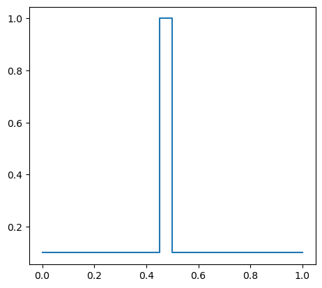
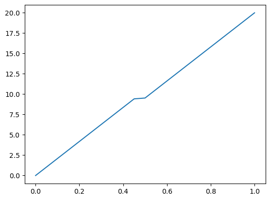
Assuming that the coefficient \(\kappa\) is element-wise constant, set a different value of the constant in the middle of the domain.
mesh = UnitIntervalMesh(20)  # 20 is number of intervals Omega is divided into
cell = mesh.ufl_cell()
plot(mesh)

elem = FiniteElement("Lagrange", cell, 1)
W = FunctionSpace(mesh, elem)

# kappa = Constant(1.0)
k_elem = FiniteElement("DG", mesh.ufl_cell(), 0)
kappa_e = Function(FunctionSpace(mesh, k_elem))
kappa_e.vector()[:] = 0.1
kappa_e.vector()[9] = 1
print(kappa_e.vector()[:])
plot(kappa_e)
Calling FFC just-in-time (JIT) compiler, this may take some time.
[0.1 0.1 0.1 0.1 0.1 0.1 0.1 0.1 0.1 1.  0.1 0.1 0.1 0.1 0.1 0.1 0.1 0.1
 0.1 0.1]
[<matplotlib.lines.Line2D at 0x7f8de986fc70>]
v = TestFunction(W)
u = TrialFunction(W)

a = kappa_e * dot(grad(u), grad(v)) * dx  # left hand side of our equation
S = Constant(0.0)  # source term
L = S * v * dx  # right hand side of our equation

value_left = Constant(0.0)
value_right = Constant(20.0)
# Imposing Dirichlet BC to the left boundary node
bc_l = DirichletBC(W, value_left, "on_boundary && near(x[0], 0)")
# Imposing Dirichlet BC to the right boundary node
bc_r = DirichletBC(W, value_right, "on_boundary && near(x[0], 1)")
bcs = [bc_l, bc_r]   # list of boundary conditions to apply to the problem

uh = Function(W)  # place to store the solution
solve(a == L, uh, bcs)  # solve the problem
plot(uh)
Calling FFC just-in-time (JIT) compiler, this may take some time.
Solving linear variational problem.
[<matplotlib.lines.Line2D at 0x7f8de9a2ece0>]
Exercice 2: Playing with the source term#
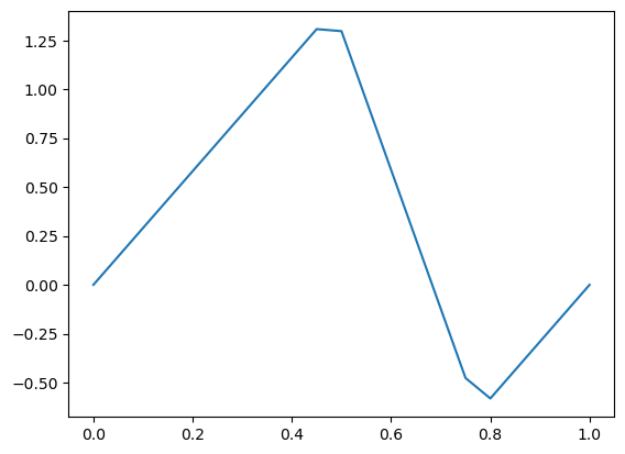
Let’s do the same with the source term. Let’s include a source term of the given value at the same element within the domain.
# S = Constant(0.0) # source term
s_elem = FiniteElement("DG", interval, 0)
S_e = Function(FunctionSpace(mesh, s_elem))
S_e.vector()[:] = 0  # set all the vector entries to 1.0
S_e.vector()[9] = 20  # set the 10th entry to 20.0
S_e.vector()[15] = -20  # set the 16th entry to -20.0
print(S_e.vector()[:])


L = S_e * v * dx  # right hand side of our equation

value_left = Constant(0.0)
value_right = Constant(0.0)
# Imposing Dirichlet BC to the left boundary node
bc_l = DirichletBC(W, value_left, "on_boundary && near(x[0], 0)")
# Imposing Dirichlet BC to the right boundary node
bc_r = DirichletBC(W, value_right, "on_boundary && near(x[0], 1)")
bcs = [bc_l, bc_r]   # list of boundary conditions to apply to the problem

uh = Function(W)  # place to store the solution
solve(a == L, uh, bcs)  # solve the problem
plot(uh)
[  0.   0.   0.   0.   0.   0.   0.   0.   0.  20.   0.   0.   0.   0.
   0. -20.   0.   0.   0.   0.]
Calling FFC just-in-time (JIT) compiler, this may take some time.
Solving linear variational problem.
[<matplotlib.lines.Line2D at 0x7f8de98d4e20>]
FEniCS: Moving to 2D#
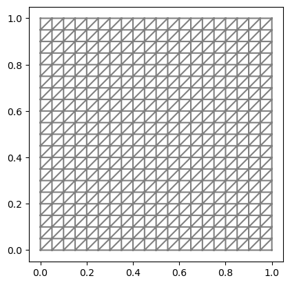
Adding the second dimension is straight forward using FEniCS. Only minor changes have to made on defining the mesh, the FunctionSpace, and the boundaries of the 2D domain.
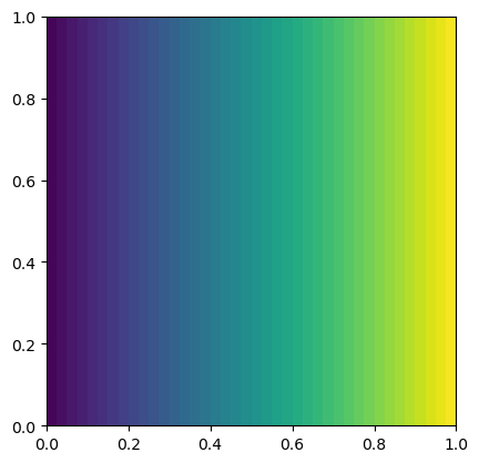
mesh = UnitSquareMesh(20, 20)
plot(mesh)
[<matplotlib.lines.Line2D at 0x7f8de9785f90>,
 <matplotlib.lines.Line2D at 0x7f8de9786200>]
elem = FiniteElement("Lagrange", mesh.ufl_cell(), 1)
W = FunctionSpace(mesh, elem)

kappa = Constant(1.0)
S = Constant(0.0)

v = TestFunction(W)  # the test function
# the TrialFunction is basically a symbol representing the unknown
u = TrialFunction(W)

a = kappa * dot(grad(u), grad(v)) * dx  # left hand side of our equation
S = Constant(0.0)  # source term
L = S * v * dx  # right hand side of our equation

value_left = Constant(0.0)
value_right = Constant(2.0)
# Imposing Dirichlet BC to the left boundary node
bc_l = DirichletBC(W, value_left, "on_boundary && near(x[0], 0)")
# Imposing Dirichlet BC to the right boundary node
bc_r = DirichletBC(W, value_right, "on_boundary && near(x[0], 1)")
bcs = [bc_l, bc_r]   # list of boundary conditions to apply to the problem

uh = Function(W)  # place to store the solution
solve(a == L, uh, bcs)  # solve the problem
plot(uh)
Calling FFC just-in-time (JIT) compiler, this may take some time.
Calling FFC just-in-time (JIT) compiler, this may take some time.
Calling FFC just-in-time (JIT) compiler, this may take some time.
Calling FFC just-in-time (JIT) compiler, this may take some time.
Calling FFC just-in-time (JIT) compiler, this may take some time.
Calling FFC just-in-time (JIT) compiler, this may take some time.
Solving linear variational problem.
<matplotlib.tri._tricontour.TriContourSet at 0x7f8de836afe0>
Exercise: Solving a 1D transient diffusion problem#
Now that we succefully solved the diffusion equation for steady state conditions, let’s look at the time evolution of the solution before equilibrium is reached.
In this case, the equation is:
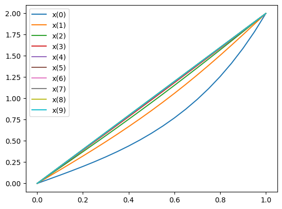
One classical approach of evaluating the time derivative term is to approximate it by means of finite differences.The following backward Euler scheme can be used:
Turning the PDE into a variational form#
As before, we express the variational form of our problem with the approximated time derivation term:
One can rearrange the equation in a way that all the unknown terms are present in the left hand side and all the known terms present in the right hand side.
FEniCS: Let’s start as before#
We first need to discretize our domain into a FE mesh. Add your code below:
# Add code here
In this code you need to introduce some new variables
dt, the time step, which is aConstantobject that appear in both the righ hand side (a) and left hand side (L) form.nb_t, that we will use to constrain the maximum number of time steps to run.u_oldaFunctionthat should hold the solution at the previous time step. NOTE: AFunctionvariable is initialized with zeros when created in Python.
FEniCS: Time loop#
Since we want to look at the time evolution of the diffusion process, we need to solve the problem step by step within a time loop and update the solution over the time step dt.
# Uncomment and modify this code
# for t in range(nb_t):
#     #
#     # Write the necessary code lines to solve the system of equations!
#     #
#     # update the old solution to the new one for next time step
#     assign(u_old, uh)
NOTE: When defining the function u_old in the variational form, FEniCS will automatically take into account the updated values in the system of equations when we execute assign(u_old, uh).
Solution#
Press below to see the solution
Show code cell source
from dolfin import *
mesh = UnitIntervalMesh(20)  # 20 is number of intervals Omega is divided into
elem = FiniteElement("CG", mesh.ufl_cell(), 1)
W = FunctionSpace(mesh, elem)

kappa = Constant(1.0)  # physical material property
S = Constant(0.0)  # source term

dt = Constant(0.2)  # time step
nb_t = 10  # number of time step - loop

v = TestFunction(W)  # the test function
# the TrialFunction is basically a symbol representing the unknown
u = TrialFunction(W)
u_old = Function(W)  # Solution at previous time step. Initialized to zero.

a = (u * v) / dt * dx + kappa * dot(grad(u), grad(v)) * \
    dx  # left hand side of our equation
L = (u_old * v) / dt * dx + S * v * dx  # right hand side of our equation

value_left = Constant(0.0)
value_right = Constant(2.0)
# Imposing Dirichlet BC to the left boundary node
bc_l = DirichletBC(W, value_left, "on_boundary && near(x[0], 0)")
# Imposing Dirichlet BC to the right boundary node
bc_r = DirichletBC(W, value_right, "on_boundary && near(x[0], 1)")

uh = Function(W)  # place to store the solution
bcs = [bc_l, bc_r]   # list of boundary conditions to apply to the problem
for t in range(nb_t):
    set_log_active(False)
    solve(a == L, uh, bcs)  # solve the the new solution
    plot(uh, label=f"x({t})")
    # update the old solution to the new one for next time step
    assign(u_old, uh)
plt.legend()
Show code cell output
Calling FFC just-in-time (JIT) compiler, this may take some time.
Calling FFC just-in-time (JIT) compiler, this may take some time.
<matplotlib.legend.Legend at 0x7f8de98b9510>
Improving the time dependent code#
Above you have been able to solve the time-dependent heat equation. However, when calling solve(a==L, uh, bcs), there is a lot of things happening under the hood.
We assemble the left hand side into a matrix
A. This matrix is time-independent and should be assembled only once. However, when callingsolvewe re-assemble it at every time step.We assemble the right hand side. This is time dependent (since it depends on
u_old, and should be assembe at every time step.)Apply boundary conditions. This has to be done once for the matrix, and on every time step for the right hand side
Solve the linear problem. We can use a LU-decomposition method to solve the linear system
Ax=b. As the matrix is time-independent, we can cache the LU-decomposition.
For the time independent problem, we can write it as
mesh = UnitIntervalMesh(10)
elem = FiniteElement("Lagrange", mesh.ufl_cell(), 1)
W = FunctionSpace(mesh, elem)

kappa = Constant(1.0)
S = Constant(0.0)

v = TestFunction(W)  # the test function
# the TrialFunction is basically a symbol representing the unknown
u = TrialFunction(W)

a = kappa * dot(grad(u), grad(v)) * dx  # left hand side of our equation
S = Constant(0.0)  # source term
L = S * v * dx  # right hand side of our equation

value_left = Constant(0.0)
value_right = Constant(2.0)
# Imposing Dirichlet BC to the left boundary node
bc_l = DirichletBC(W, value_left, "on_boundary && near(x[0], 0)")
# Imposing Dirichlet BC to the right boundary node
bc_r = DirichletBC(W, value_right, "on_boundary && near(x[0], 1)")
bcs = [bc_l, bc_r]   # list of boundary conditions to apply to the problem

uh = Function(W)  # place to store the solution
A = assemble(a)  # Assemble bilinear form a into a matrix
b = assemble(L)  # Assemble the linear form into a vector
for bc in bcs:  # For each bc apply the boundary condition to the matrix and vector
    bc.apply(A)
    bc.apply(b)
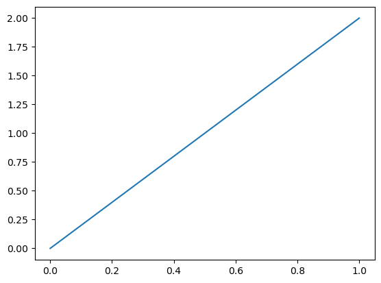
solver = LUSolver(A)  # Create an LU solver
solver.solve(uh.vector(), b)  # Solve problem
plot(uh)
Calling FFC just-in-time (JIT) compiler, this may take some time.
Calling FFC just-in-time (JIT) compiler, this may take some time.
Calling FFC just-in-time (JIT) compiler, this may take some time.
Calling FFC just-in-time (JIT) compiler, this may take some time.
Calling FFC just-in-time (JIT) compiler, this may take some time.
Calling FFC just-in-time (JIT) compiler, this may take some time.
[<matplotlib.lines.Line2D at 0x7f8de80c9d80>]
Solving a transient 2D diffusion problem#
Turning the PDE into a variational problem#
Once we rearrange the unknown terms in the left hand side and the known terms in the right hand side, we obtain:
Exercise 2: Solve a 2D transient diffusion problem#
# Add code solving the 2D transient diffusion problem here
Solution#
Press below to see the solution
Show code cell source
# 20 is number of intervals Omega is divided into
mesh = UnitSquareMesh(20, 20)
# here interval is a FEniCS builtin representing a single interval
elem = FiniteElement("Lagrange", mesh.ufl_cell(), 1)
W = FunctionSpace(mesh, elem)

kappa = Constant(1.0)  # physical material property
S = Constant(0.0)  # source term

dt = Constant(0.1)  # time step
nb_t = 25  # number of time step - loop

v = TestFunction(W)  # the test function
# the TrialFunction is basically a symbol representing the unknown
u = TrialFunction(W)
u_old = Function(W)  # Solution at previous time step. Initialized to zero.


a = (u * v) / dt * dx + kappa * dot(grad(u), grad(v)) * \
    dx  # left hand side of our equation
L = (u_old * v) / dt * dx + S * v * dx  # right hand side of our equation

value_left = Constant(0.0)
value_right = Constant(2.0)
# Imposing Dirichlet BC to the left boundary node
bc_l = DirichletBC(W, value_left, "on_boundary && near(x[0], 0)")
# Imposing Dirichlet BC to the right boundary node
bc_r = DirichletBC(W, value_right, "on_boundary && near(x[0], 1)")
bcs = [bc_l, bc_r]   # list of boundary conditions to apply to the problem

uh = Function(W)  # place to store the solution

A = assemble(a)
for bc in bcs:
    bc.apply(A)

solver = LUSolver(A)
for t in range(nb_t):
    b = assemble(L)  # Reassemble L on every time step
    for bc in bcs:  # RE-apply bc to b
        bc.apply(b)
    solver.solve(uh.vector(), b)  # Solve on given time step
    assign(u_old, uh)


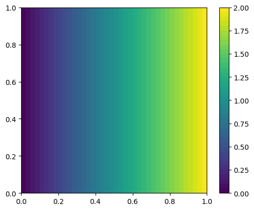
fig = plt.figure()
im = plot(uh)
fig.colorbar(im)
Show code cell output
Calling FFC just-in-time (JIT) compiler, this may take some time.
Calling FFC just-in-time (JIT) compiler, this may take some time.
Calling FFC just-in-time (JIT) compiler, this may take some time.
Calling FFC just-in-time (JIT) compiler, this may take some time.
Calling FFC just-in-time (JIT) compiler, this may take some time.
Calling FFC just-in-time (JIT) compiler, this may take some time.
<matplotlib.colorbar.Colorbar at 0x7f8de80d3760>
Extra material (application of Dirichlet conditions)#
Where did the boundary terms go, and when can I ignore them?#
To make it clear what is happening with the boundary terms we ignored, what FEniCS does behind the scenes is the following:
mesh = UnitIntervalMesh(5)  # 20 is number of intervals Omega is divided into
# here interval is a FEniCS builtin representing a single interval
elem = FiniteElement("Lagrange", mesh.ufl_cell(), 1)
W = FunctionSpace(mesh, elem)

v = TestFunction(W)  # the test function
# the TrialFunction is basically a symbol representing the unknown
u = TrialFunction(W)

kappa = Constant(1.0)
a = kappa * dot(grad(u), grad(v)) * dx  # left hand side of our equation
S = Constant(0.0)  # source term
L = S * v * dx  # right hand side of our equation

value_left = Constant(0.0)
value_right = Constant(2.0)
# Imposing Dirichlet BC to the left boundary node
bc_l = DirichletBC(W, value_left, "on_boundary && near(x[0], 0)")
# Imposing Dirichlet BC to the right boundary node
bc_r = DirichletBC(W, value_right, "on_boundary && near(x[0], 1)")

A = assemble(a)
b = assemble(L)
print("\nBefore BCs are applied without bdy term: \n")
from sympy import init_printing, Matrix, Eq
init_printing(use_latex = 'mathjax') # Used to print Latex to the screen
%matplotlib inline

(Matrix(A.array()), Matrix(b.get_local()))
Before BCs are applied without bdy term:
bc_l.apply(A)
bc_r.apply(A)
bc_l.apply(b)
bc_r.apply(b)

print("\nAfter BCs are applied without bdy term: \n")

(Matrix(A.array()), Matrix(b.get_local()))
After BCs are applied without bdy term:
This tells you how DirichletBCs are applied in FEniCS, and why adding the boundary terms wouldn’t matter. When you give FEniCS a boundary condition, it replaces the equation it got from putting \(v=\phi_i\) for the right \(i\) by one reading \(u_i = \) the value \(u\) is supposed to have there, meaning a row of \(A\) is replaced by one with a single 1 and the rest 0, and the correponding part of \(b\) set to the right value.
Note that you are only allowed to ignore the boundary terms when you have a boundary condition of the form \(u = \) constant at every part of the boundary. Such boundary conditions are called Dirichlet boundary conditions. Sometimes you might have conditions involving the derivative of \(u\) instead. Those are called Neumann or Robin boundary conditions, and generally mean you have to add a term to rhs.
If you had wanted to add boundary terms, this could be done as follows:
a = kappa * dot(grad(u), grad(v)) * dx + u.dx(0) * v * \
    ds  # ds means integrate over boundary
A = assemble(a)
b = assemble(L)

print("\nBefore BCs are applied with bdy term: \n",)
(Matrix(A.array()), Matrix(b.get_local()))
Calling FFC just-in-time (JIT) compiler, this may take some time.
Before BCs are applied with bdy term:
bc_l.apply(A)
bc_r.apply(A)
bc_l.apply(b)
bc_r.apply(b)

print("\nAfter BCs are applied with bdy term: \n")
(Matrix(A.array()), Matrix(b.get_local()))
After BCs are applied with bdy term:
Notice that although the matrix A becomes different when you add the boundary term, the only difference is in the first and last row, which corresponds to nodes where we have boundary conditions. This is why you can ignore the boundary term where you have a Dirichlet boundary condition.

